Ever wondered what you can do with text information and an analytical tool like R

Text analysis is a branch of data analytics concerned with the extraction of text information and insights from datasets. This makes it a useful tool in our times, as massive amounts of text are generated every minute. A good example where such analysis would easily fit is in understanding X, Facebook, or blogs. The analysis can also be stretched to examine internet traffic, say for a hotspot, if for some reason you need to monitor it.

Introduction

This post will examine a music database containing details of songs from different albums, artists, and genres.

Objectives:

Displaying the years with the most songs.
Displaying which artists have the most songs.
Displaying the longest albums.
Creating word clouds for the albums and song titles to see the most re-used words.

Preprocessing

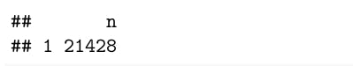
We first import the dataset, which can be found here, count the rows, and obtain the first few rows. As shown we have 21,428 songs to analyze.

music <- read.csv("~/Software/musics/output.csv")
count(music)

head(music)

Pre-processing is necessary after importing the dataset, which we perform here by checking for missing data.

cbind(lapply(lapply(music, is.na), sum))

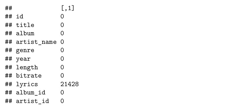
The lyrics column has no data as the empty rows match the total count of rows calculated before, so it would be sensible to get rid of it. Some other columns will also not do much for us, such as id, album_id, and artist_id. We get rid of them too.

music <- subset(music, select=-c(lyrics, id, album_id, artist_id)) head(music)

Visualizations

What's left is a clean database that we can start visualizing. The aim is to get the top 10 values by: count of the year, artist name, and length of an album.

top_10 <- music %>% count(year) %>% arrange(desc(n)) %>% top_n(10)

filtered <- music %>% 
    filter(year %in% top_10$year) 
    %>% mutate(Years = factor(year, levels=top_10$year))

ggplot(filtered, aes(x=Years)) +
geom_bar() + coord_flip() +
labs(x = "Year", y = "Count", title = "Top 10 Years by Song Count")

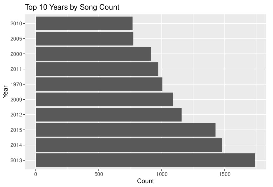
2013 leads in song counts, followed by 2014, 2015, 2012, 2009 and 1970. These years have more than 1000 songs each.

top_10_art <- music %>% 
    count(artist_name) %>% 
    arrange(desc(n)) %>% 
    top_n(10)

filtered_art <- music %>% 
    filter(artist_name %in% top_10_art$artist_name) %>% 
    mutate(Artists = factor(artist_name, levels=top_10_art$artist_name))

ggplot(filtered_art, aes(x=Artists), fill=Artists) +
    geom_bar() + coord_flip() +
    labs(x = "Artist Name", y = "Count", title = "Top 10 Artists by Song Count")

Looking at the artist counts, The Beatles lead with close to 400 songs, followed by Lil Wayne, Celine Dion, and Michael Jackson. The rest of the artists have less than 300 songs each.

album_lengths <- music %>%
  group_by(album) %>% 
  summarize(length_minutes = sum(length)/1000/60) %>% 
  arrange(desc(length_minutes)) %>% 
  top_n(10)

album_lengths$album <- factor(album_lengths$album, levels = album_lengths$album)

ggplot(album_lengths, aes(x = album, y = length_minutes)) +
  geom_bar(stat = "identity") +
  coord_flip() +
  labs(x = "Album Name", y = "Length (Minutes)", title = "Top 10 Album Lengths")

The album Swahili, Exclusive lead, followed by The Jazz Ultim, both at more than 2000 songs. Billboard albums also dominate in the number of songs, with over 500 songs each.

Word clouds

corpus <- Corpus(VectorSource(music$album))
corpus <- tm_map(corpus, content_transformer(tolower))
corpus <- tm_map(corpus, removePunctuation)
corpus <- tm_map(corpus, removeNumbers)
corpus <- tm_map(corpus, removeWords, stopwords("english"))
corpus <- tm_map(corpus, stripWhitespace)
term_doc_matrix <- TermDocumentMatrix(corpus)
word_frequency <- rowSums(as.matrix(term_doc_matrix))

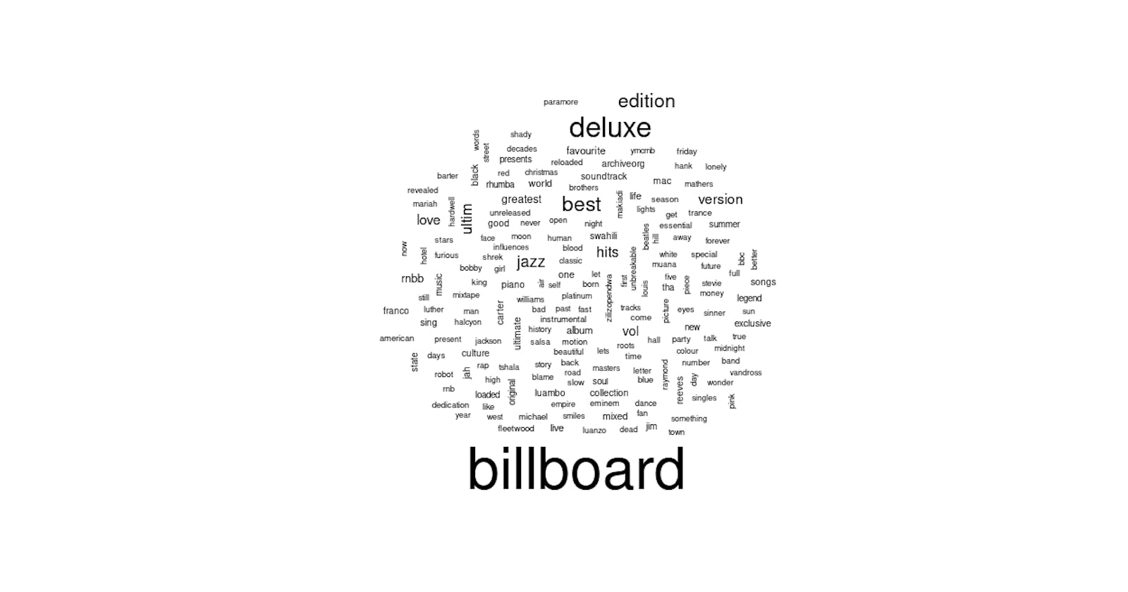
wordcloud(words = names(word_frequency), freq = word_frequency, min.freq = 40)

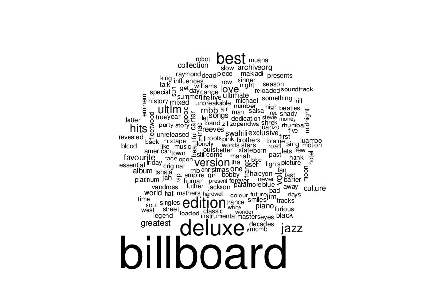
For the album name word cloud, here we observe that the words billboard, deluxe, best, edition, and jazz have the most appearances. Although these words are not descriptive, they indicate the type of albums present in the database. The word love also appears in most album names.

corpus <- Corpus(VectorSource(music$title))
corpus <- tm_map(corpus, content_transformer(tolower))
corpus <- tm_map(corpus, removePunctuation)
corpus <- tm_map(corpus, removeNumbers)
corpus <- tm_map(corpus, removeWords, stopwords("english"))
corpus <- tm_map(corpus, stripWhitespace)
term_doc_matrix <- TermDocumentMatrix(corpus)
word_frequency <-rowSums(as.matrix(term_doc_matrix))

wordcloud(words = names(word_frequency), freq = word_frequency, min.freq = 50)

For the song titles word cloud, the word love, feat, and dont lead in count. Other recognizable titles include time, heart, baby, night and world. It is safe to say that most of the songs in the database are, therefore, love songs.

Takeaways

Text analysis provides one with a powerful tool to get into the details of datasets containing textual information. This analysis can be easily expanded to other use cases, and the possibilities are only limited by one's imagination.

Have a good day.

#R #textanalysis

Collins Kasyoki